Carbonate Chemistry Examples
2023-07-29
Source:vignettes/carbonate_chemistry_examples.Rmd
carbonate_chemistry_examples.RmdThis vignette provides examples of the carbonate chemistry tools implemented by the microbialkitchen package to explore carbonate solubility and pH control in open and closed media systems. See the carbonate chemistry equations vignette for conceptual background.
CO2 solubility
solubilities <- tibble(
  temperature = seq(from = 0, to = 40, by = 5) %>% qty("C"),
  solubility = calculate_gas_solubility("CO2", temperature)
)

solubilities %>%
  ggplot() +
  aes(temperature, solubility) +
  geom_line(size = 2) +
  scale_x_qty(unit = "C") +
  theme_bw()
## Warning: Using `size` aesthetic for lines was deprecated in ggplot2 3.4.0.
## ℹ Please use `linewidth` instead.
## This warning is displayed once every 8 hours.
## Call `lifecycle::last_lifecycle_warnings()` to see where this warning was
## generated.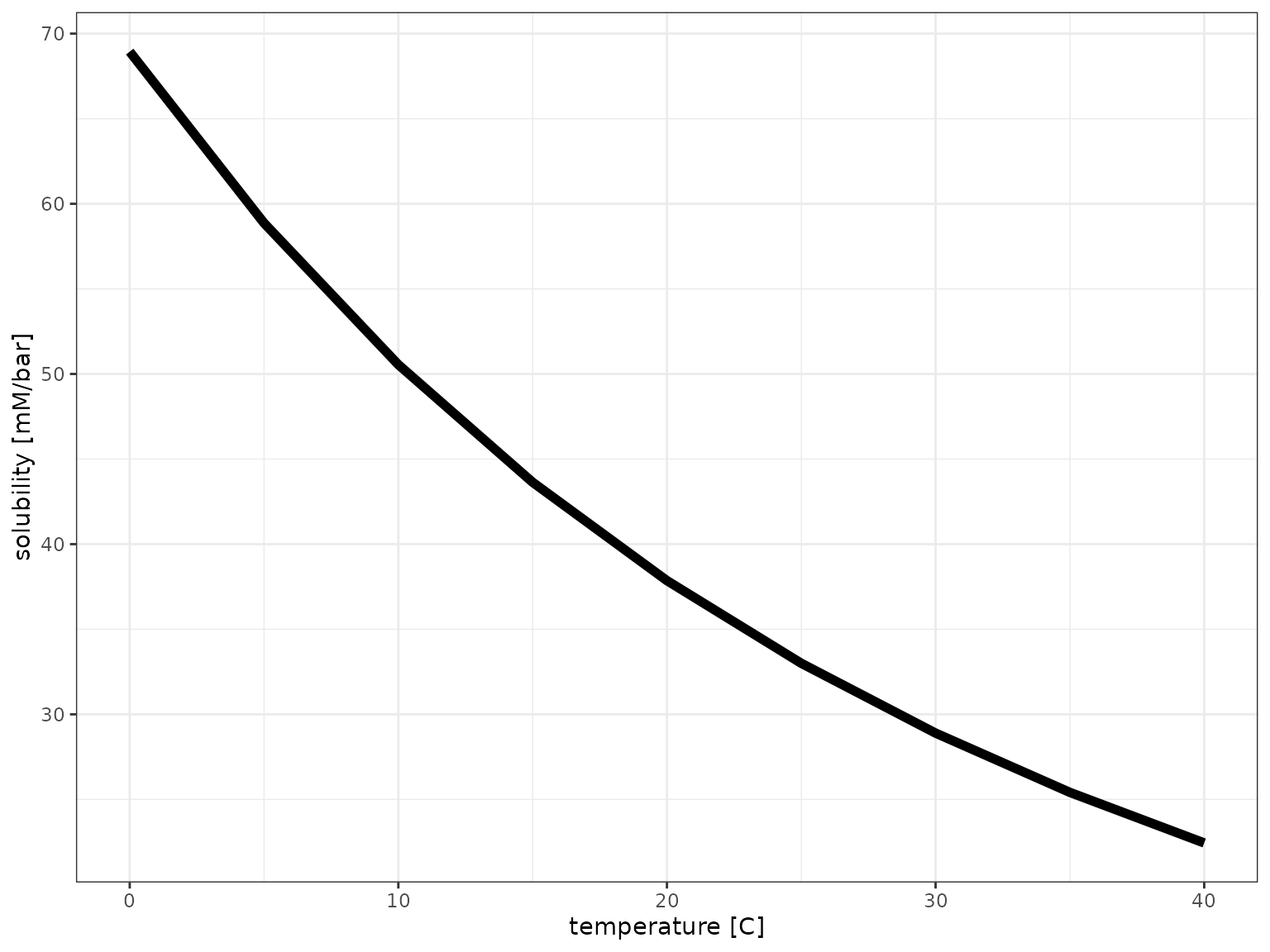
Speciation
# calculate
df_speciation <-
  tibble(
    pH = seq(3, 14, by = 0.1),
    DIC = qty(10, "mM"),
    `H2CO3*` = calculate_carbonic_acid(pH, DIC = DIC),
    HCO3 = calculate_bicarbonate(pH, DIC = DIC),
    CO3 = calculate_carbonate(pH, DIC = DIC)
  )

# visualize
df_speciation %>%
  # pivoting longer for the concentration columns
  pivot_longer(
    names_to = "Species", values_to = "Concentration",
    cols = c(`H2CO3*`, HCO3, CO3)
  ) %>%
  ggplot() +
  aes(pH, Concentration, color = Species) +
  geom_line() +
  scale_x_continuous(expand = c(0, 0), breaks = c(1:14)) +
  scale_y_qty(each = TRUE) +
  theme_bw()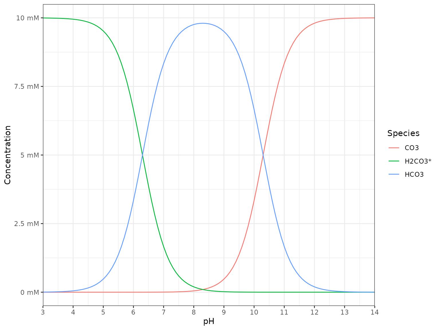
Open system
CO2 only
# range of pCO2s
pCO2s <- tibble(
  pCO2 = qty(c(seq(0, 5, by=0.1), seq(5, 20, by=1), seq(20, 200, by=5)), "mbar")
)
# range of temperature
temperatures <- tibble(
  temperature = qty(c(10, 25, 37), "C")
)

# calculate for all combinations
df_pH_vs_pCO2 <-
  crossing(pCO2s, temperatures) %>%
  mutate(
    pH = calculate_open_system_pH(pCO2, temp = temperature),
    DIC = calculate_DIC(pH, pCO2, temp = temperature),
    CO2 = calculate_ideal_gas_molarity(pCO2, temp = temperature)
  )
df_pH_vs_pCO2 %>%
  # pivoting longer mixed data types requires explicit units first
  make_qty_units_explicit(DIC = "mM", CO2 = "mM") %>%
  pivot_longer(
    cols = c(pH, `DIC [mM]`, `CO2 [mM]`),
    names_to = "var", values_to = "value"
  ) %>%
  filter(!(var == "pH" & value > 5.5)) %>%
  mutate(temperature = as_factor(temperature, unit = "C")) %>%
  ggplot() +
  aes(pCO2, value, color = temperature) +
  geom_line() +
  scale_x_qty(expand = c(0, 0)) +
  scale_color_brewer(palette = "Set1") +
  facet_grid(var~., scales = "free_y") +
  expand_limits(x = 0) +
  theme_bw() +
  labs(y = NULL)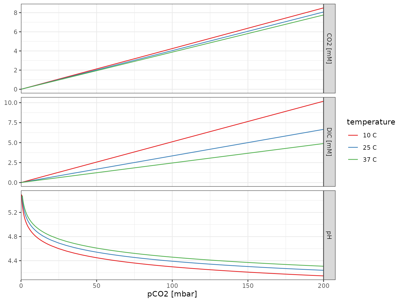
Adjusting pH with alkalinity
# to calculate how much base (NaOH or NaHCO3) to add
calculate_open_system_alkalinity(pH = 6.8, pCO2 = qty(0.4, "mbar"))
## <mk_molarity_concentration[1]>
## [1] 41.67307
calculate_open_system_alkalinity(pH = 6.8, pCO2 = qty(50, "mbar"))## <mk_molarity_concentration[1]>
## [1] 5.220963
calculate_open_system_alkalinity(pH = 6.8, pCO2 = qty(200, "mbar"))## <mk_molarity_concentration[1]>
## [1] 20.88414
# to calculate pH with addition of a specific amount of base
calculate_open_system_pH(pCO2 = qty(0.4, "mbar"), alkalinity = qty(5, "mM"))
## [1] 8.848121
calculate_open_system_pH(pCO2 = qty(50, "mbar"), alkalinity = qty(5, "mM"))## [1] 6.781229
calculate_open_system_pH(pCO2 = qty(200, "mbar"), alkalinity = qty(5, "mM"))## [1] 6.179416
# to calculate pH with addition of a specific amount of acid
calculate_open_system_pH(pCO2 = qty(0.4, "mbar"), alkalinity = qty(-1, "nM"))
## [1] 5.589293
calculate_open_system_pH(pCO2 = qty(50, "mbar"), alkalinity = qty(-1, "nM"))## [1] 4.541239
calculate_open_system_pH(pCO2 = qty(200, "mbar"), alkalinity = qty(-1, "nM"))## [1] 4.240209Visualization
# range of pCO2s
pCO2s <- tibble(pCO2 = qty(c(0.4, 50, 200), "mbar"))
# range of temperature
temperatures <- tibble(temperature = qty(c(25, 37), "C"))

# calculate for all combinations
zero <- qty(0, "mM")
df_base_vs_pH <-
  crossing(pCO2s, temperatures, pH = seq(3, 7.5, by = 0.05)) %>%
  mutate(
    ions = calculate_open_system_alkalinity(pH, pCO2, temp = temperature),
    `Add base (e.g. NaOH)` = case_when(ions > zero ~ ions, TRUE ~ zero),
    `Add acid (e.g. HCl)` = case_when(ions < zero ~ -1*ions, TRUE ~ zero),
    DIC = calculate_DIC(pH, pCO2, temp = temperature)
  )

p <- df_base_vs_pH %>%
  pivot_longer(
    cols = c(`Add base (e.g. NaOH)`, `Add acid (e.g. HCl)`, `DIC`),
    names_to = "var", values_to = "concentration"
  ) %>%
  filter(concentration > zero) %>%
  mutate(
    temperature = as_factor(temperature, unit = "C"),
    panel = as_factor(pCO2, unit = "mbar")
  ) %>%
  ggplot() +
  aes(pH, concentration, color = var, linetype = temperature) +
  geom_vline(xintercept = 7, color = "black", size = 1) +
  geom_line() +
  scale_x_continuous(breaks = 1:14, expand = c(0, 0)) +
  scale_y_qty(each = TRUE) +
  scale_color_brewer("Component", palette = "Set1") +
  facet_wrap(~panel, nrow = 1, scales = "free_y") +
  theme_bw()
p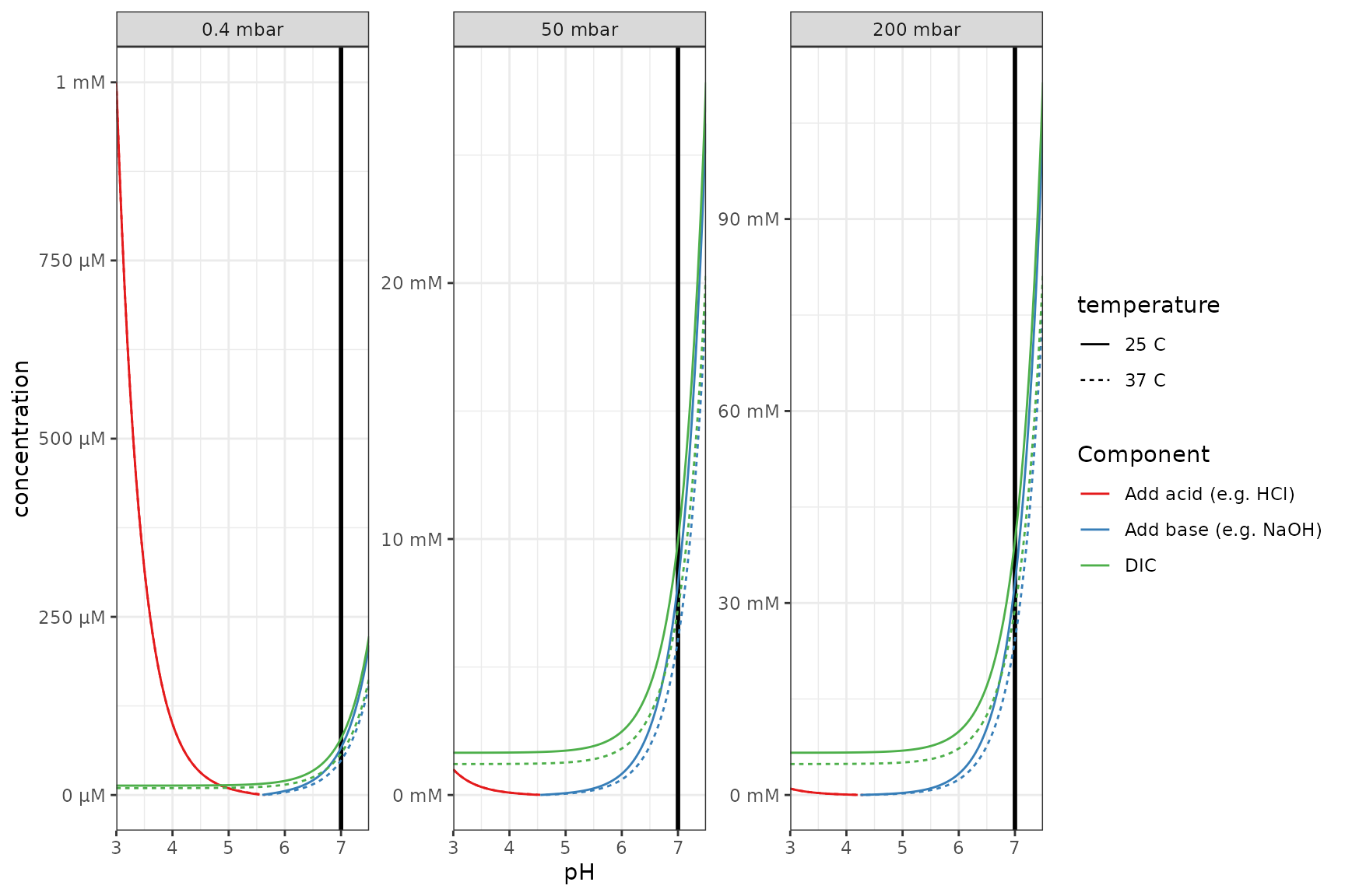
Log scale
# easier to see in log space and equal y axis + a vertical line
p_log <- p +
  scale_y_qty(each = TRUE, trans = "log10") +
  facet_wrap(~panel, nrow = 1)
## Scale for y is already present.
## Adding another scale for y, which will replace the existing scale.
p_log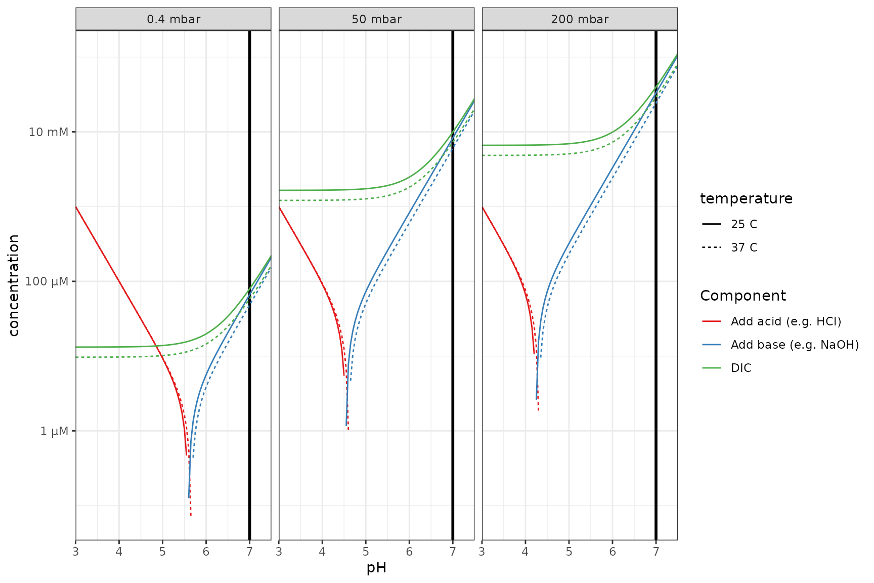
Adjusting pH with a buffer
For simplicty keeping temperature constant at the default (25C).
buffer <- qty(c(1, 10, 50), "mM")
# to calculate how much base (NaOH or NaHCO3) to add
df <- tibble(
  buffer = buffer,
  add = calculate_open_system_alkalinity(
    pH = 6.8,
    pCO2 = qty(50, "mbar"),
    buffer = buffer,
    buffer_pKa = 7.5
  )
)
df
## # A tibble: 3 × 2
## buffer add
## <mk_mlrt_> <mk_mlrt_>
## 1 1 5.39
## 2 10 6.88
## 3 50 13.5
# what if buffer is mono-sodium? (negative means HCl or other strong acid required instead of base)
df %>% mutate(add_if_salt_buffer = add - buffer)
## # A tibble: 3 × 3
## buffer add add_if_salt_buffer
## <mk_mlrt_> <mk_mlrt_> <mk_mlrt_>
## 1 1 5.39 4.39
## 2 10 6.88 -3.12
## 3 50 13.5 -36.5
# to calculate pH with addition of a specific buffer
df %>%
  mutate(
    pH = calculate_open_system_pH(
      pCO2 = qty(50, "mbar"),
      buffer = buffer,
      alkalinity = add,
      buffer_pKa = 7.5
    )
  )
## # A tibble: 3 × 3
## buffer add pH
## <mk_mlrt_> <mk_mlrt_> <dbl>
## 1 1 5.39 6.80
## 2 10 6.88 6.80
## 3 50 13.5 6.80Different concentrations of weak acid (same pKa)
# range of pCO2s
pCO2s <- tibble(pCO2 = qty(c(0.4, 50, 200), "mbar"))
# range of buffers
buffers <- tibble(
  buffer = qty(c(0, 20, 20, 20, 50), "mM"),
  buffer_pKa = c(7.5, 7.5, 9, 6, 7.5)
)

# calculate for all combinations
df_base_w_buffer_vs_pH <-
  crossing(pCO2s, buffers, pH = seq(3, 7.5, by = 0.05)) %>%
  mutate(
    ions = calculate_open_system_alkalinity(pH, pCO2, buffer = buffer, buffer_pKa = buffer_pKa),
    `Add base (e.g. NaOH)` = case_when(ions > zero ~ ions, TRUE ~ zero),
    `Add acid (e.g. HCl)` = case_when(ions < zero ~ -1*ions, TRUE ~ zero),
    DIC = calculate_DIC(pH, pCO2)
  )

# visualize
plot_df <- df_base_w_buffer_vs_pH %>%
  pivot_longer(
    cols = c(`Add base (e.g. NaOH)`, `Add acid (e.g. HCl)`, `DIC`),
    names_to = "var", values_to = "concentration"
  ) %>%
  mutate(
    panel = as_factor(pCO2, unit = "mbar"),
    Buffer = sprintf("%s (pkA=%s)", buffer, buffer_pKa)
  ) %>%
  filter(concentration > zero)

p_log %+%
  filter(plot_df, buffer_pKa == 7.5) %+%
  aes(linetype = Buffer) +
  labs(title = "Different concentrations of a weak acid buffer")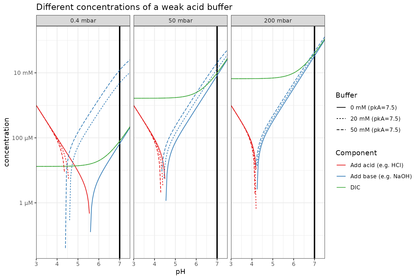
Same concentration of weak acid (different pKa)
p_log %+%
  filter(plot_df, buffer == qty(20, "mM")) %+%
    aes(linetype = Buffer) +
    labs(title = "Same concentration of a weak acid buffer with different pKa")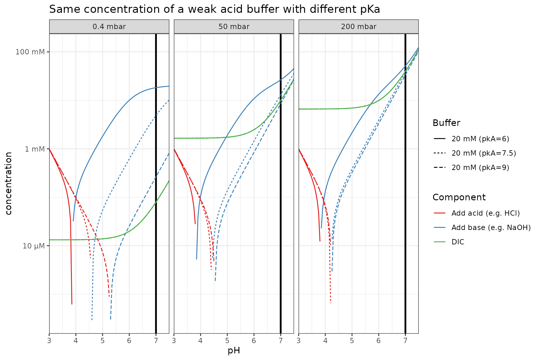
Different concentration of salt buffer (same pKa)
If the buffer is a salt instead of an acid, it contributes to the alkalinity.
plot_df2 <-
  crossing(pCO2s, buffers, pH = seq(3, 7.5, by = 0.05)) %>%
  mutate(
    ions = calculate_open_system_alkalinity(pH, pCO2, buffer = buffer, buffer_pKa = buffer_pKa) - buffer,
    `Add base (e.g. NaOH)` = case_when(ions > zero ~ ions, TRUE ~ zero),
    `Add acid (e.g. HCl)` = case_when(ions < zero ~ -1*ions, TRUE ~ zero),
    DIC = calculate_DIC(pH, pCO2)
  ) %>%
  pivot_longer(
    cols = c(`Add base (e.g. NaOH)`, `Add acid (e.g. HCl)`, `DIC`),
    names_to = "var", values_to = "concentration"
  ) %>%
  mutate(
    panel = as_factor(pCO2, unit = "mbar"),
    buffer = sprintf("%s (pkA=%s)", buffer, buffer_pKa)
  ) %>%
  filter(concentration > zero)

p_log %+%
  filter(plot_df2, buffer_pKa == 7.5) %+%
  aes(linetype = buffer) +
  labs(title = "Different concentrations of a mono-valent salt buffer")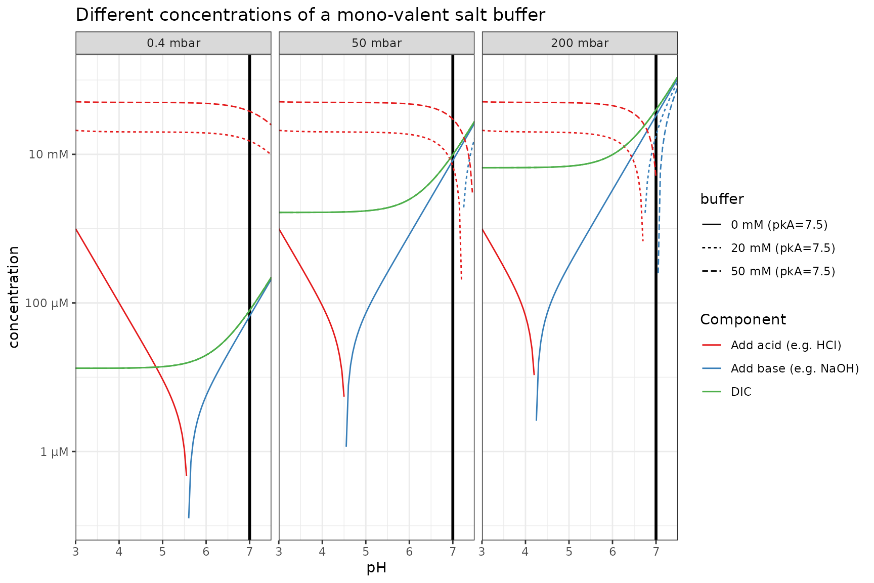
pH difference upon atmosphere switching
A rare environmental but common laboratory scenario is the sometimes unexpected change in pH upon shifting from standard atmospheric CO2 (400ppm, let’s face reality…) to some artifical higher CO2 atmosphere without adjusting anything else.
df_pH_switch <-
  df_base_w_buffer_vs_pH %>%
  filter(get_qty_value(pCO2, "mbar") == 0.4) %>%
  rename(init_pCO2 = pCO2) %>%
  crossing(pCO2 = qty(c(50, 200), "mbar")) %>%
  mutate(
    `new pH` = calculate_open_system_pH(
      pCO2 = pCO2, buffer = buffer, buffer_pKa = buffer_pKa, alkalinity = ions
    ),
    `pH difference` = `new pH` - pH,
    panel = as_factor(pCO2, unit = "mbar")
  ) %>%
  pivot_longer(
    cols = c(`new pH`, `pH difference`),
    names_to = "var", values_to = "value",
  )

p %+%
  mutate(df_pH_switch, buffer = as_factor(buffer)) %+%
  aes(y = value, color = buffer, linetype = as_factor(buffer_pKa)) +
  facet_grid(var~panel, scales = "free_y") +
  scale_color_brewer(palette = "Set1") +
  scale_linetype_manual(values = c(2, 1, 3)) +
  labs(linetype = "pKa", y = "")
## Scale for colour is already present.
## Adding another scale for colour, which will replace the existing scale.
Closed system
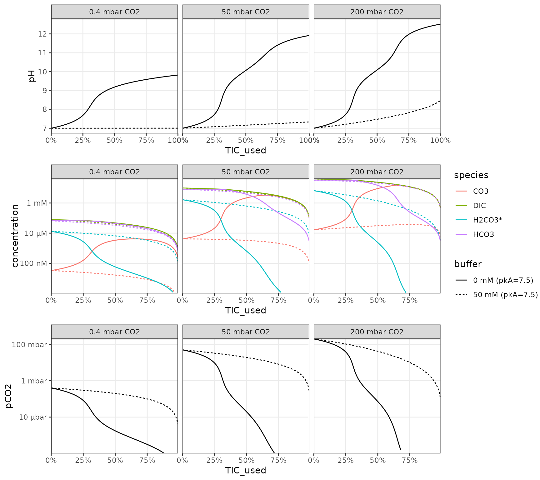
CO2 consumption
Scenario: media is equilibrated with an initial CO2 pressure and adjusted to a specific starting pH (which requires the appropriate addition of alkalinity) in presence or absence of a pH buffer. Then the vessel is closed off and has a starting total inorganic carbon from its headspace and liquid that can then be consumed. Here a few parameters are explored but additional variation will arise from changes in buffer concentration, pKa and the proportion of headspace to liquid.
df_CO2_consumption <-
  crossing(
    tibble(
      # initial medium
      pH_start = 7,
      pCO2_start = qty(c(0.4, 50, 200), "mbar")
    ),
    tibble(
      # buffer
      buffer = qty(c(0, 50), "mM"),
      pKa = 7.5
    )
  ) %>%
  mutate(
    # required alkalinity for pH
    pH_start = 7,
    alkalinity = calculate_open_system_alkalinity(
      pH = pH_start, pCO2 = pCO2_start,
      buffer = buffer, buffer_pKa = pKa),
    # close off
    V_liquid = qty(10, "mL"),
    V_gas = qty(10, "mL"),
    TIC_start = calculate_closed_system_TIC(pH = pH_start, pCO2 = pCO2_start, V_liquid = V_liquid, V_gas = V_gas)
  ) %>%
  # range of TIC used up (%)
  crossing(TIC_used = seq(0, 1, by = 0.01)) %>%
  # calculation of system at each point
  mutate(
    TIC = TIC_start * (1-TIC_used),
    pH = calculate_closed_system_pH(
      TIC = TIC, V_liquid = V_liquid, V_gas = V_gas,
      alkalinity = alkalinity, buffer = buffer, buffer_pKa = pKa),
    pCO2 = calculate_closed_system_pCO2(pH = pH, TIC = TIC, V_liquid = V_liquid, V_gas = V_gas),
    DIC = calculate_DIC(pH, pCO2 = pCO2),
    `H2CO3*` = calculate_carbonic_acid(pH, DIC = DIC),
    HCO3 = calculate_bicarbonate(pH, DIC = DIC),
    CO3 = calculate_carbonate(pH, DIC = DIC)
  ) %>%
   mutate(
    pCO2_start = as_factor(sprintf("%s CO2", pCO2_start)),
    buffer = sprintf("%s (pkA=%s)", buffer, pKa),
  )

# visualize
p_base <-
  df_CO2_consumption %>%
  ggplot() +
  aes(TIC_used, linetype = buffer) +
  scale_y_qty(each = TRUE, trans = "log10", expand = c(0, 0)) +
  scale_x_continuous(
    labels = function(x) sprintf("%.0f%%", 100*x),
    expand = c(0, 0)) +
  facet_wrap(~pCO2_start) +
  theme_bw() + theme(panel.grid.minor = element_blank()) +
  labs("TIC consumed")

p_IC <- p_base %+%
  aes(y = concentration, color = species) +
  geom_line(
    data = function(df)
      df %>% pivot_longer(
        cols = c(DIC, `H2CO3*`, HCO3, CO3),
        names_to = "species",
        values_to = "concentration",
      ) %>% filter(concentration > qty(1, "nM"))
  )

p_pH <- p_base %+%
  aes(y = pH, color = NULL) +
  geom_line() +
  scale_y_continuous() +
  theme(legend.position = "none")

p_CO2 <- p_base %+%
  aes(y = pCO2, color = NULL) +
  geom_line(data = function(df) filter(df, pCO2 > qty(1e-7, "bar"))) +
  theme(legend.position = "none")

library(cowplot)
plot_grid(p_pH, p_IC, p_CO2, ncol = 1, align = "v", axis = "lr")
CO2 production
Scenario: media with organic substrate (e.g. a sugar) is adjusted to an initial starting pH (which requires the appropriate addition of alkalinity) in presence or absence of a pH buffer. Then the vessel is closed off and CO2 is produced from the organic substrate (assuming the entire organic pool is respirable).
df_CO2_production <-
  crossing(
    tibble(
      # initial medium
      pH_start = 7,
      Corg = qty(c(1, 10, 100), "mM") # respirable carbon molarity
    ),
    tibble(
      # buffer
      buffer = qty(c(0, 50), "mM"),
      pKa = 7.5
    )
  ) %>%
  mutate(
    # required alkalinity for pH adjustment
    pH_start = 7,
    pCO2_start = qty(0.4, "mbar"), # atmospheric
    alkalinity = calculate_open_system_alkalinity(
      pH = pH_start, pCO2 = pCO2_start,
      buffer = buffer, buffer_pKa = pKa),
    # close off
    V_liquid = qty(10, "mL"),
    V_gas = qty(10, "mL"),
    TIC_start = calculate_closed_system_TIC(pH = pH_start, pCO2 = pCO2_start, V_liquid = V_liquid, V_gas = V_gas)
  ) %>%
  # range of organics respired (%)
  crossing(Corg_used = seq(0, 1, by = 0.01)) %>%
  # calculation of system at each point
  mutate(
    TIC = TIC_start + Corg * V_liquid * Corg_used,
    pH = calculate_closed_system_pH(
      TIC = TIC, V_liquid = V_liquid, V_gas = V_gas,
      alkalinity = alkalinity, buffer = buffer, buffer_pKa = pKa),
    pCO2 = calculate_closed_system_pCO2(pH = pH, TIC = TIC, V_liquid = V_liquid, V_gas = V_gas),
    DIC = calculate_DIC(pH, pCO2 = pCO2),
    `H2CO3*` = calculate_carbonic_acid(pH, DIC = DIC),
    HCO3 = calculate_bicarbonate(pH, DIC = DIC),
    CO3 = calculate_carbonate(pH, DIC = DIC)
  ) %>%
  mutate(
    Corg = as_factor(sprintf("%s org. C", Corg)),
    buffer = sprintf("%s (pkA=%s)", buffer, pKa),
  )

# plots
p_IC_b <- p_IC %+% df_CO2_production %+% aes(x = Corg_used) + facet_wrap(~Corg) +
  labs(x = "Organic C consumed")
p_pH_b <- p_pH %+% df_CO2_production %+% aes(x = Corg_used) + facet_wrap(~Corg) +
  labs(x = "Organic C consumed")
p_CO2_b <- p_CO2 %+% df_CO2_production %+% aes(x = Corg_used) + facet_wrap(~Corg) +
  labs(x = "Organic C consumed")

plot_grid(p_pH, p_IC, p_CO2, ncol = 1, align = "v", axis = "lr")